Output File Format
One of the key features of TCTrack is its output file format. Whilst all of the codes wrapped provide output data in a custom formats with minimal or zero metadata, TCTrack, by contrast, provides data in a standardised results format across all codes that is compliant with the CF-Conventions for metadata.
These pages describe the contents of this file and how it can be used downstream.
CF-Conventions and FAIR Data
The CF (Climate and Forecast) Conventions for NetCDF data are best introduced in their own words:
“The CF metadata conventions are designed to promote the processing and sharing of files created with the NetCDF API. The conventions define metadata that provide a definitive description of what the data in each variable represents, and the spatial and temporal properties of the data. This enables users of data from different sources to decide which quantities are comparable, and facilitates building applications with powerful extraction, regridding, and display capabilities.”
TCTrack produces CF-compliant files for all tracking algorithms with clear metadata.
FAIR is an acronym for Findable, Accessible, Interoperable, and Reusable. It outlines expectations for high-quality metadata and standards-compliant file formats. By providing clear variable definitions, provenance information, and following established conventions, such datasets enable robust scientific workflows, reproducibility, and integration into a wide range of analysis tools. This approach maximizes the scientific value of the data and supports transparent, collaborative research. It also ensures that datasets and files are meaningful, useable, and reliable, even when shared standalone or a significant time after generation.
Overview
Each NetCDF output file produced by the to_netcdf() method of a Tracker
contains a collection of tropical cyclone trajectories, with each trajectory representing
a single storm track.
The format follows the
CF Conventions: H4 Trajectory Data
recommendations for trajectory data using two-dimensional arrays of
shape (n_trajectory, n_observation).
Any trajectories shorter than n_observations end with fill values.
File Format
Dimensions
trajectory: Number of detected storm tracks (each a unique trajectory).
Has a corresponding dimension coordinate variable indicating the trajectory index
observation Maximum number of time steps (observations) in the trajectories.
Has a corresponding dimension coordinate variable indicating the observation index
Variables
Required variables
These coordinate variables are always present in a dataset:
trajectory: Unique index for each trajectory.
Dimensions:
(trajectory)Dimension coordinate.
Designated by the
cf_role="trajectory_id"attribute.
observation: Index for each observation within a trajectory.
Dimensions:
(observation)Dimension coordinate.
time: Time of each observation.
Dimensions:
(trajectory, observation)Auxiliary coordinate.
Attributes include
unitsandcalendaramongst others
latitude: Latitude of the observation.
Dimensions:
(trajectory, observation)Auxiliary coordinate.
longitude: Longitude of the observation.
Dimensions:
(trajectory, observation)Auxiliary coordinate.
Optional variables
A number of additional variables may also be written to file for each trajectory depending on the algorithm, data used, and user-configuration. Most commonly these will be measures of “intensity” along the tracks, but may also include auxilliary coordinates such as grid indices.
Intensity variables
Dimensions:
(trajectory, observation)Attributes should include
unitsand may also provide a CF cell method indicating how the variable was calculated.
Ancillary Field Variables
Files always include two Ancillary status flag variables:
start_flag
Dimensions:
(trajectory)
end_flag
Dimensions:
(trajectory)
These indicate any tracks that start or end within 1 day of the input dataset bounds and may therefore extend outside this range.
Global Attributes
Files contain a number of global metadata attributes
Conventions: Indicates the version of the CF-conventions the file was generated with
featureType:
trajectory, a CF attribute aiding data processing and regognition of data formattctrack_version: Attribute detailing the software version used to generate the file. Indicates semantic version and commit hash.
tctrack_tracker: Tracker name identifying the algorithm used (e.g., TSTORMSTracker)
<TCTrack-Tracker>_parameters: JSON-encoded dictionaries recording all key parameters used for detection and tracking, to aid reproducibility.
Inspection and Usage
As a CF-compliant NetCDF file TCTrack outputs can be accessed using a number of downstream tools and softwares including NetCDF-Python, xarray, cf-python etc. both within and beyond the Python ecosystem.
Perhaps the quickest way of inspecting the metadata is to use the ncdump utility:
ncdump -h my_tctrack_output.nc
netcdf my_tctrack_output {
dimensions:
        trajectory = 2 ;
        observation = 13 ;
variables:
        int64 trajectory(trajectory) ;
                trajectory:standard_name = "trajectory" ;
                trajectory:cf_role = "trajectory_id" ;
                trajectory:long_name = "trajectory index" ;
        int64 observation(observation) ;
                observation:standard_name = "observation" ;
                observation:long_name = "observation index" ;
        double time(trajectory, observation) ;
                time:standard_name = "time" ;
                time:long_name = "time" ;
                time:units = "days since 1950-01-01 12:00:00.000000" ;
                time:missing_value = -100000000. ;
                time:calendar = "360_day" ;
        double latitude(trajectory, observation) ;
        ...
Here we show how to inspect a file using cf-python which highlights the structure described above:
import cf

# Read the input file. This automatically concatenates in time.
fieldlist = cf.read("my_tctrack_output.nc")

for field in fieldlist:
    field.dump()
------------------------------------------------------------------
Field: air_pressure_at_sea_level (ncvar%air_pressure_at_sea_level)
------------------------------------------------------------------
Conventions = 'CF-1.12'
detect_parameters = '{"u_in_file": "u_ref_interpolated_final.nc", "v_in_file":
                     "v_ref_interpolated_final.nc", "vort_in_file":
                     "vort850_interpolated_final.nc", "tm_in_file":
                     "tm_interpolated_final.nc", "slp_in_file":
                     "slp_interpolated_final.nc", "use_sfc_wind": true,
                     "vort_crit": 3.5e-05, "tm_crit": 0.0, "thick_crit": 50.0,
                     "dist_crit": 4.0, "lat_bound_n": 70.0, "lat_bound_s":
                     -70.0, "do_spline": false, "do_thickness": false}'
featureType = 'trajectory'
long_name = 'Sea Level Pressure'
missing_value = np.float64(-10000000000.0)
standard_name = 'air_pressure_at_sea_level'
stitch_parameters = '{"r_crit": 900.0, "wind_crit": 17.0, "vort_crit": 3.5e-05,
                     "tm_crit": 0.5, "thick_crit": 50.0, "n_day_crit": 2,
                     "do_filter": true, "lat_bound_n": 40.0, "lat_bound_s":
                     -40.0, "do_spline": false, "do_thickness": false}'
tctrack_tracker = 'TSTORMSTracker'
tctrack_version = '0.1.dev157+g482a888b7'
tstorms_parameters = '{"tstorms_dir": "/home/jwa34/rds/hpc-
                      work/TSTORMS_clean/tropical_storms_pub/", "output_dir":
                      "/home/jwa34/rds/rds-inspire-tc-
                      TqEGHMWTn8A/test_data/tstorms/output_test/", "input_dir":
                      "/rds/project/rds-TqEGHMWTn8A/test_data/tstorms"}'
units = 'Pa'

Data(trajectory(2), observation(13)) = [[1002.11, ..., nan]] Pa

Cell Method: area: maximum (lesser circle of radius 4.0 degrees)

Field Ancillary: status_flag
    long_name = 'Trajectory starting at start of dataset flag.'
    standard_name = 'status_flag'
    Data(trajectory(2)) = [0, 0]

Field Ancillary: status_flag
    long_name = 'Trajectory finishing at end of dataset flag.'
    standard_name = 'status_flag'
    Data(trajectory(2)) = [0, 0]

Domain Axis: observation(13)
Domain Axis: trajectory(2)

Dimension coordinate: trajectory
    cf_role = 'trajectory_id'
    long_name = 'trajectory index'
    standard_name = 'trajectory'
    Data(trajectory(2)) = [0, 1]

Dimension coordinate: observation
    long_name = 'observation index'
    standard_name = 'observation'
    Data(observation(13)) = [0, ..., 12]

Auxiliary coordinate: time
    calendar = '360_day'
    long_name = 'time'
    missing_value = np.float64(-100000000.0)
    standard_name = 'time'
    units = 'days since 1950-01-01 12:00:00.000000'
    Data(trajectory(2), observation(13)) = [[1950-01-06 00:00:00, ..., -275828-03-21 12:00:00]] 360_day

Auxiliary coordinate: latitude
    long_name = 'latitude'
    missing_value = np.float64(-999.9)
    standard_name = 'latitude'
    units = 'degrees_north'
    Data(trajectory(2), observation(13)) = [[-9.26, ..., nan]] degrees_north

Auxiliary coordinate: longitude
    long_name = 'longitude'
    missing_value = np.float64(-999.9)
    standard_name = 'longitude'
    units = 'degrees_east'
    Data(trajectory(2), observation(13)) = [[67.32, ..., nan]] degrees_east

...
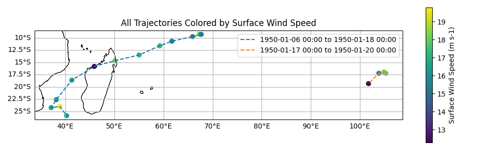
Plotting example
Tracks can be visualised using variety of softwares. Here we demonstrate a simple example using NetCDF with cartopy, though users may also explore cf-python, xarray, or hurucanpy.
import netCDF4
import numpy as np
import matplotlib.pyplot as plt
import cartopy.crs as ccrs

# Open the NetCDF file
with netCDF4.Dataset("my_tctrack_output.nc") as ncfile:
    # Read variables
    lat_var = ncfile.variables["latitude"]
    lon_var = ncfile.variables["longitude"]
    time_var = ncfile.variables["time"]
    intensity_var = ncfile.variables["wind_speed"]
    traj_var = ncfile.variables["trajectory"]

    lats = lat_var[:]
    lons = lon_var[:]
    intensity = intensity_var[:]
    traj_labels = traj_var[:]
    times = time_var[:]

    # Convert times to datetime objects
    missing_time = getattr(time_var, "missing_value", np.nan)
    times = np.ma.masked_where(times == missing_time, times)
    time_units = getattr(time_var, "units")
    time_calendar = getattr(time_var, "calendar")
    times_dt = netCDF4.num2date(times, units=time_units, calendar=time_calendar)

    # Get intensity metadata for labels
    intensity_name = getattr(intensity_var, "long_name")
    intensity_units = getattr(intensity_var, "units", "")
    min_intensity = np.nanmin(intensity)
    max_intensity = np.nanmax(intensity)

    plt.figure(figsize=(10, 6))
    ax = plt.axes(projection=ccrs.PlateCarree())
    ax.coastlines()
    ax.gridlines(draw_labels=True)

    # Plot each trajectory
    for i in traj_labels:
        times_i = times_dt[i, :].compressed()
        label = (
            f"{times_i[0].strftime('%Y-%m-%d %H:%M')} to "
            f"{times_i[-1].strftime('%Y-%m-%d %H:%M')}"
        )
        pl = ax.plot(
            lons[i], lats[i], "--", transform=ccrs.PlateCarree(), label=f"{label}"
        )
        sc = ax.scatter(
            lons[i],
            lats[i],
            c=intensity[i],
            cmap="viridis",
            s=40,
            vmin=min_intensity,
            vmax=max_intensity,
            transform=ccrs.PlateCarree(),
        )

    plt.colorbar(sc, label=f"{intensity_name} ({intensity_units})")
    plt.title(f"All Trajectories Colored by {intensity_name}")
    plt.legend()
    plt.savefig("my_tracks.png")